Quick peak fitting

This cell below is if you have already loaded in some 1d data, and can then select specific peaks to carry out a peak fitting routine on. First create a set of peaks you want to use in the fit following the format

peak1 = {'type':name-of-peak,
         'settings':
            {'center':[6.25,6.2,6.3],
             'sigma': [0.02,1e-6,0.1],
             'amplitude': [7,1e-6,18],
             'fraction':[0.15,0,1]}
         }

The currently supported peak type names are listed below, and use built-in models within the lmfit python package - click on the links below to find out more about the available settings for each peak type

• "pvoigt": fits using PseudoVoigtModel,

• "gaussian": fits using GaussianModel,

• "lorentzian": fits using LorentzianModel,

• "split_lorentzian": fits using SplitLorentzianModel,

• "skewed_gaussian": fits using SkewedGaussianModel,

from giwaxs_toolbox.processing import data_loader
from giwaxs_toolbox.plotting import reset_plots
import matplotlib.pyplot as plt
from pprint import pprint
import numpy as np
import os

folder1="/dls/science/groups/das/ExampleData/i07/fast_rsm_example_data/tests_versioned/v2.4.1_i07_2026-04-14"
filelist= [file for file in os.listdir(folder1) if file.endswith('.hdf5')]

#create your data loader for your data directory path
loader=data_loader(datafolder=folder1)

#choose which datasets you want to load

example_ivqfiles=['IvsQ_432196_2026-04-14_14h19m06s.hdf5',
                  'IvsQ_610009_2026-04-14_14h22m41s.hdf5']

# load the files into a results object
ivqresults=loader.loadfiles(example_ivqfiles)

from giwaxs_toolbox.processing import peakfit_and_plot


peak1 = {'type':'pvoigt',
         'settings':
            {'center':[6.25,6.2,6.3],
             'sigma': [0.02,1e-6,0.05],
             'amplitude': [7,1e-6,18000],
             'fraction':[0.15,0,1]}
         }

peak2 = {'type':'pvoigt',
         'settings':
            {'center':[5.38,5.35,5.39],
             'sigma': [0.02,1e-6,0.05],
             'amplitude': [7,1e-6,1800],
             'fraction':[0.15,0,1]}
         }
peaklist=[peak1]
#peaklist=[peak1,peak2]


res=ivqresults[0]
q=res.x_axis
intensity=res.data
con1=q>6.15
con2=q<6.35
selection=con1&con2
x=q[selection]
y=intensity[selection]
report=peakfit_and_plot(peaklist,x,y)

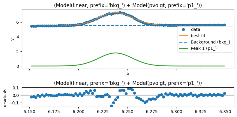
This will use your selected profile, along with the limits gived by constraints con1 and con2, to fit the peaks detailed in peaklist - with the fitting result saved to the report object, and a summary plot being output

You can access the details of the fit by calling the report object

report

Fit Result

Model: (Model(linear, prefix='bkg_') + Model(pvoigt, prefix='p1_'))

Fit Statistics

fitting method	leastsq
# function evals	130
# data points	93
# variables	6
chi-square	0.13232665
reduced chi-square	0.00152100
Akaike info crit.	-597.622556
Bayesian info crit.	-582.426959
R-squared	0.99573762

Parameters

name	value	standard error	relative error	initial value	min	max	vary	expression
bkg_slope	0.54498482	0.07742226	(14.21%)	10.0	-inf	inf	True
bkg_intercept	2.14131480	0.48801746	(22.79%)	5.466299057006836	-inf	inf	True
p1_amplitude	0.07662386	0.00325009	(4.24%)	7.0	1.0000e-06	18000.0000	True
p1_center	6.23801411	1.4548e-04	(0.00%)	6.25	6.20000000	6.30000000	True
p1_sigma	0.02019399	1.9587e-04	(0.97%)	0.02	1.0000e-06	0.05000000	True
p1_fraction	5.1531e-13	0.00432395	(839096239403.65%)	0.15	0.00000000	1.00000000	True
p1_fwhm	0.04038798	3.9174e-04	(0.97%)	0.04	-inf	inf	False	2.0000000*p1_sigma
p1_height	1.78229547	124.957295	(7011.03%)	156.45256423122214	-inf	inf	False	(((1-p1_fraction)*p1_amplitude)/max(1e-15, (p1_sigma*sqrt(pi/log(2))))+(p1_fraction*p1_amplitude)/max(1e-15, (pi*p1_sigma)))

Correlations (unreported values are < 0.100)

Parameter1	Parameter 2	Correlation
bkg_slope	bkg_intercept	-0.9997
p1_amplitude	p1_fraction	+0.9726
bkg_intercept	p1_amplitude	-0.3562
bkg_slope	p1_amplitude	+0.3359
bkg_intercept	p1_fraction	-0.3174
bkg_slope	p1_fraction	+0.2980
bkg_slope	p1_center	-0.2484
bkg_intercept	p1_center	+0.2484
p1_sigma	p1_fraction	-0.2465

alternatively you can access individual results like this:

report.params['p1_fwhm'].value

0.04038797932363416

report.params['p1_center'].value

6.23801411075692

fitting peaks to a stack of profiles

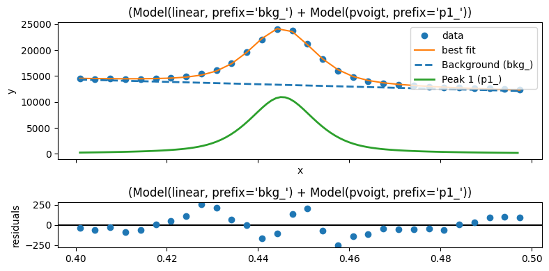
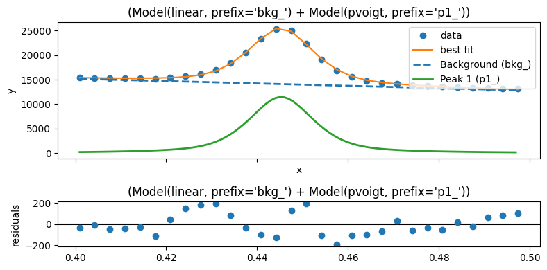
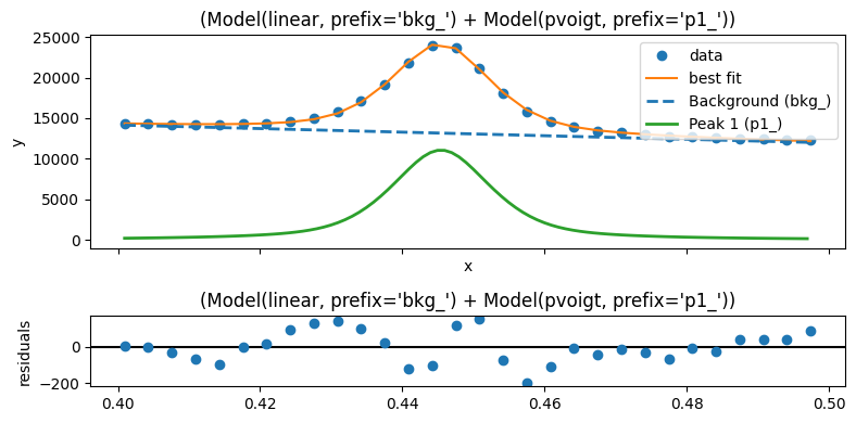
You can run similar parameters for multiple profiles, by loading multiple profiles and then looping over the fitting routine. Below multiple slices from one dataset are loaded in and then each profile is fitted with a similar peak.

#choose which datasets you want to load

example_ivqfiles=['IvsQ_536350_2026-04-14_14h20m34s.hdf5']*10

# load the files into a results object
ivqresults=loader.loadfiles(example_ivqfiles, index1vals=np.arange(0,100,10))

len(ivqresults)

10

peak1 = {'type':'pvoigt',
         'settings':
            {'center':[0.44,0.42,0.5],
             'sigma': [0.02,1e-6,0.05],
             'amplitude': [7,1e-6,18000],
             'fraction':[0.15,0,1]}
         }
peaklist=[peak1]
result_list=[]
for i in np.arange(10):
    res=ivqresults[i]
    q=res.x_axis
    intensity=res.data
    con1=q>0.4
    con2=q<0.5
    selection=con1&con2
    x=q[selection]
    y=intensity[selection]
    report=peakfit_and_plot(peaklist,x,y)
    result_list.append(report)

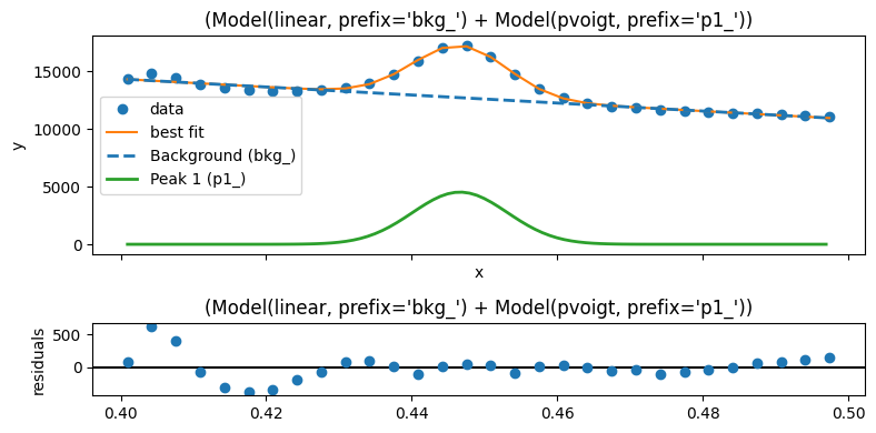
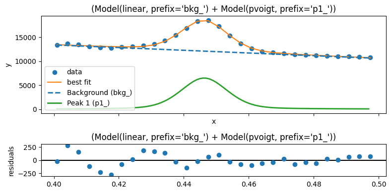
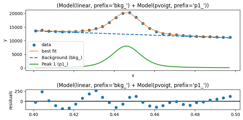
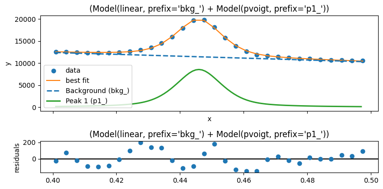
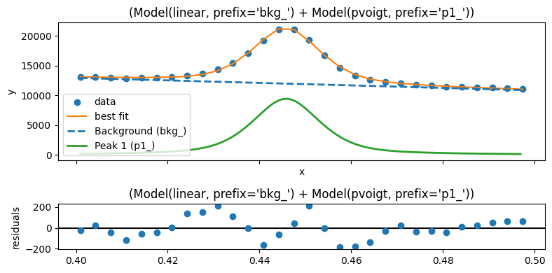
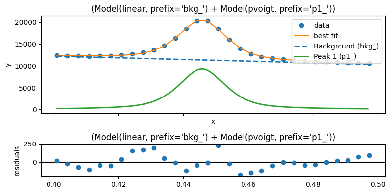
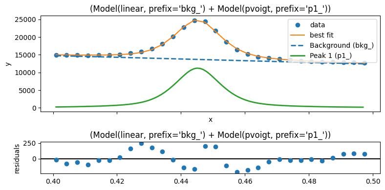
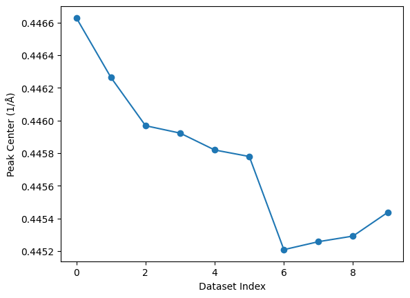
You can then select out the fitted parameters you are interested and visualise them on a plot

centre_values = [result.params['p1_center'].value for result in result_list]
plt.plot(centre_values, marker='o')
plt.xlabel('Dataset Index')
plt.ylabel('Peak Center (1/Å)')

Text(0, 0.5, 'Peak Center (1/Å)')