i22 Corrections#
Installation#
To run this notebook locally, first clone the git repository and install the python dependencies as shown below:
git clone https://github.com/DiamondLightSource/adcorr.git
cd adcorr
pip install -e .[dev,docs] -r requirements.txt
Alternatively, you may wish to clone the repository and open the project in a container with Visual Studio Code and the Remote Containers extension (ms-vscode-remote.remote-containers).
Import dependencies#
[1]:
from math import prod
from pathlib import Path

from h5py import File
from numpy import array, ones

from adcorr.corrections import mask_frames
from adcorr.sequences import pauw_dispersed_sample_sequence

from matplotlib.pyplot import imshow, subplots
from matplotlib.colors import LogNorm
Matplotlib is building the font cache; this may take a moment.
Download i22 tutorial dataset#
In this tutorial we will use the PEG dataset included in the Diamond Light Source i22 Tutorial Dataset, hosted on zenodo: https://zenodo.org/record/2671750
Please download this file and extract it; Once complete please set the SAMPLE_PATH, DISPERSANT_PATH and BACKGROUND_PATH to the locations of the i22-363095.nxs, i22-363096.nxs and i22-363098.nxs files respectively.
The PEG dataset contains a series of NeXus files corresponding to individual experimental captures, by reading the entry1/title entry of each we can deduce that they have the following correspondence:
i22-363095.nxs: Empty capillary tubei22-363096.nxs: Water in capillary tubei22-363098.nxs-i22-363107.nxs: PEG in water (varying concentrations)
[2]:
SAMPLE_PATH =  Path("/tmp/I22 Tutorial Dataset/I22 PEG Tutorial/i22-363105.nxs")
DISPERSANT_PATH = Path("/tmp/I22 Tutorial Dataset/I22 PEG Tutorial/i22-363096.nxs")
BACKGROUND_PATH = Path("/tmp/I22 Tutorial Dataset/I22 PEG Tutorial/i22-363095.nxs")
Load required data from files#
We shall now extract all available requisite data from the available NeXus files.
From each the sample, dispersant and background files we will load the following:
Image stack, from
entry1/Pilatus2M_WAXS/dataCount times, from
entry1/instrument/Pilatus2M_WAXS/count_timeIncident flux, from
entry1/I0/dataTransmitted flux, from
entry1/It/data
Additionally, we will extract the following data from solely the sample NeXus file:
Pixel wise mask, from
entry1/Pilatus2M_WAXS/pixel_maskBeam center x & y, from
entry1/instrument/Pilatus2M_WAXS/beam_center_x&entry1/instrument/Pilatus2M_WAXS/beam_center_yrespectivelyPhysical pixel sizes in x & y, from
entry1/instrument/Pilatus2M_WAXS/x_pixel_size&entry1/instrument/Pilatus2M_WAXS/y_pixel_sizerespectivelyDistance between sample and detector, from
entry1/instrument/Pilatus2M_WAXS/distanceSample thickness, from
entry1/sample/thickness
[3]:
with File(SAMPLE_PATH) as sample_file:
    print(f"Retrieving sample from {array(sample_file['entry1/title'])}")
    frames = array(sample_file["entry1/Pilatus2M_WAXS/data"])
    frames_count_times = array(sample_file["entry1/instrument/Pilatus2M_WAXS/count_time"])
    frames_incident_flux = array(sample_file["entry1/I0/data"])
    frames_transmitted_flux = array(sample_file["entry1/It/data"])

    mask = array(sample_file["entry1/Pilatus2M_WAXS/pixel_mask"])
    beam_center_x = array(sample_file["entry1/instrument/Pilatus2M_WAXS/beam_center_x"])
    beam_center_y = array(sample_file["entry1/instrument/Pilatus2M_WAXS/beam_center_y"])
    x_pixel_size = array(sample_file["entry1/instrument/Pilatus2M_WAXS/x_pixel_size"])
    y_pixel_size = array(sample_file["entry1/instrument/Pilatus2M_WAXS/y_pixel_size"])
    sample_detector_separation = array(sample_file["entry1/instrument/Pilatus2M_WAXS/distance"])
    sample_thickness = array(sample_file["entry1/sample/thickness"])

with File(DISPERSANT_PATH) as dispersant_file:
    print(f"Retrieving dispersant from {array(dispersant_file['entry1/title'])}")
    dispersants = array(dispersant_file["entry1/Pilatus2M_WAXS/data"])
    dispersants_count_times = array(dispersant_file["entry1/instrument/Pilatus2M_WAXS/count_time"])
    dispersants_incident_flux = array(dispersant_file["entry1/I0/data"])
    dispersants_transmitted_flux = array(dispersant_file["entry1/It/data"])

with File(BACKGROUND_PATH) as background_file:
    print(f"Retrieving background from {array(background_file['entry1/title'])}")
    backgrounds = array(background_file["entry1/Pilatus2M_WAXS/data"])
    backgrounds_count_times = array(background_file["entry1/instrument/Pilatus2M_WAXS/count_time"])
    backgrounds_incident_flux = array(background_file["entry1/I0/data"])
    backgrounds_transmitted_flux = array(background_file["entry1/It/data"])
Retrieving sample from b'PEG in water (80:20 v/v)'
Retrieving dispersant from b'Water in capillary tube'
Retrieving background from b'Empty capillary tube'
Prepare data for processing#
Re-shape & scale loaded data#
Prior to correction, we must re-shape and scale the loaded data to fit out requisite dimensionality and units.
For each the sample, dispersant and background we will apply the following re-shaping:
Image stacks will be reshaped to three dimensions (
NumFrames,FrameWidth,FrameHeight)Count times will be flattened to a one dimensional array
Incident flux will be flattened to a one dimensional array
Transmitted flux will be flattened to a one dimensional array
Additionally, we will extract the singular value in each the beam center, pixel size and thickness arrays and convert them to a scalar value.
Finally, we will perform the following scaling:
Incident flux will be scaled from milli-counts to counts
Transmitted flux will be scaled from micro-counts to counts
Sample thickness will be scaled from milli-metres to metres
[4]:
frames = frames.reshape(prod(frames.shape[:-2]), *frames.shape[-2:])
frames_count_times = frames_count_times.flatten()
frames_incident_flux = frames_incident_flux.flatten() * 1e-3
frames_transmitted_flux = frames_transmitted_flux.flatten() * 1e-6

dispersants = dispersants.reshape(prod(dispersants.shape[:-2]), *dispersants.shape[-2:])
dispersants_count_times = dispersants_count_times.flatten()
dispersants_incident_flux = dispersants_incident_flux.flatten() * 1e-3
dispersants_transmitted_flux = dispersants_transmitted_flux.flatten() * 1e-6

backgrounds = backgrounds.reshape(prod(backgrounds.shape[:-2]), *backgrounds.shape[-2:])
backgrounds_count_times = backgrounds_count_times.flatten()
backgrounds_incident_flux = backgrounds_incident_flux.flatten() * 1e-3
backgrounds_transmitted_flux = backgrounds_transmitted_flux.flatten() * 1e-6

beam_center_pixels = (
    beam_center_y.item(),
    beam_center_x.item()
)
pixel_sizes = (
    x_pixel_size.item(),
    y_pixel_size.item()
)
sample_thickness = sample_thickness.item() * 1e-3
Add additional fields#
Several required fields are not available from the downloaded datasets, as such we will have to provide constants, as follows:
FLATFIELDis assigned a uniform field of ones, as flatfield correction has been applied by the detectorMINIMUM_PULSE_SEPARATIONis assigned a value of 2μs, this is typical for a photon counting detectorMINIMUM_ARRIVAL_SEPARATIONis assigned a value of 3μs, this is typical for a photon counting detectorBASE_DARK_CURRENTis assigned a value of zero, as we have no information on itTEMPORAL_DARK_CURRENTis assigned a value of zero, as we have no information on itFLUX_DEPENDANT_DARK_CURRENTis assigned a value of zero, as we have no information on itSENSOR_ABSORPTION_COEFFICIENTis assigned a value of 0.85, this is typical for a silicone based sensorSENSOR_THICKNESSis assigned a value of 1mm, this is typical for a silicone based photon counting detectorBEAM_POLARIZATIONis assigned a value of 0.5, representing unpolarized lightDISPLACED_FRACTIONis assigned a value of 0.8, as shown in theentry1/titlefield of the sample file
[5]:
FLATFIELD = ones(frames.shape[-2:])
MINIMUM_PULSE_SEPARATION = 2e-6
MINIMUM_ARRIVAL_SEPARATION = 3e-6
BASE_DARK_CURRENT = 0.0
TEMPORAL_DARK_CURRENT = 0.0
FLUX_DEPENDANT_DARK_CURRENT = 0.0
SENSOR_ABSORPTION_COEFFICIENT = 0.85
SENSOR_THICKNESS = 1e-3
BEAM_POLARIZATION = 0.5
DISPLACED_FRACTION = 0.8
Visualize raw data#
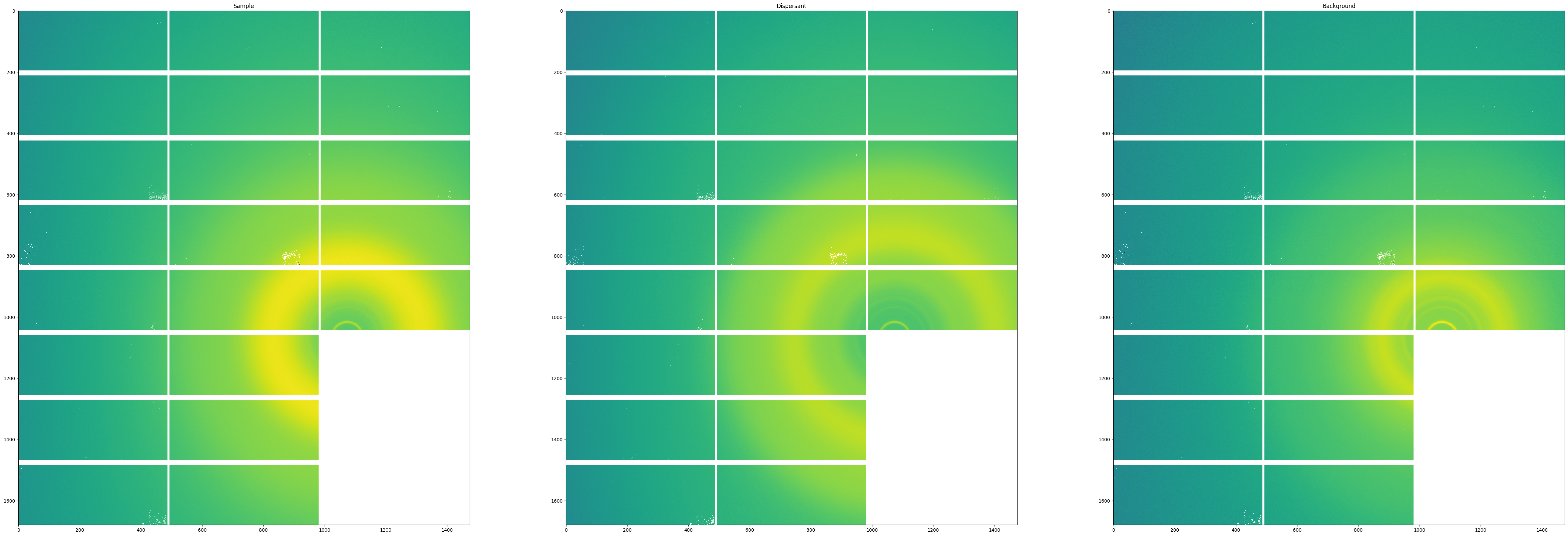
As a sanity check, we will visualize the first image from the images stack of each the sample, dispersant and background datasets, with the pixelwise mask applied.
[6]:
fig, axes = subplots(1, 3)
fig.set_size_inches(60,20)
axes[0].imshow(mask_frames(frames, mask)[0], norm=LogNorm(), interpolation="none")
axes[0].title.set_text("Sample")
axes[1].imshow(mask_frames(dispersants, mask)[0], norm=LogNorm(), interpolation="none")
axes[1].title.set_text("Dispersant")
axes[2].imshow(mask_frames(backgrounds, mask)[0], norm=LogNorm(), interpolation="none")
axes[2].title.set_text("Background")
Correct data using Pauw dispersed sample sequence#
We will now apply the dispersed sample data correction sequence described by Pauw et al. (2017) [https://doi.org/10.1107/S1600576717015096] by calling the pauw_dispersed_sample_sequence with all requisite parameters. The resultant corrected images will be stored in the corrected_frames variable for subsequent visualization.
[7]:
corrected_frames = pauw_dispersed_sample_sequence(
    frames,
    dispersants,
    backgrounds,
    mask,
    FLATFIELD,
    frames_count_times,
    dispersants_count_times,
    backgrounds_count_times,
    frames_incident_flux,
    frames_transmitted_flux,
    dispersants_incident_flux,
    dispersants_transmitted_flux,
    backgrounds_incident_flux,
    backgrounds_transmitted_flux,
    MINIMUM_PULSE_SEPARATION,
    MINIMUM_ARRIVAL_SEPARATION,
    BASE_DARK_CURRENT,
    TEMPORAL_DARK_CURRENT,
    FLUX_DEPENDANT_DARK_CURRENT,
    beam_center_pixels,
    pixel_sizes,
    sample_detector_separation,
    SENSOR_ABSORPTION_COEFFICIENT,
    sample_thickness,
    SENSOR_THICKNESS,
    BEAM_POLARIZATION,
    DISPLACED_FRACTION,
)
Visualize corrected data#
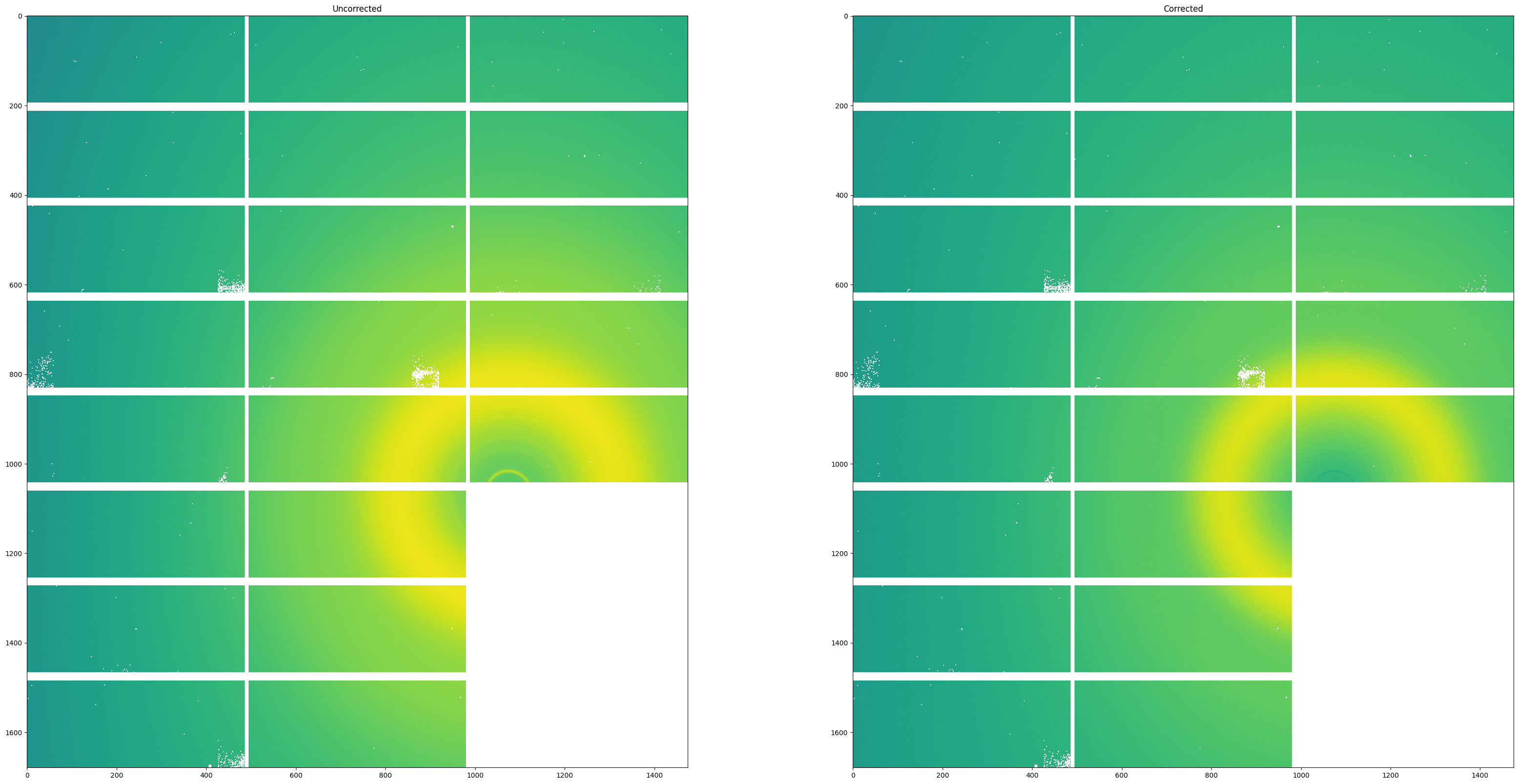
Finally, we will visualize both the first image of the uncorrected sample image stack beside the first image of the corrected image stack. As you can see, several artifacts due to the beam are removed including most notably the small Kapton ring near the beam center.
[8]:
fig, axes = subplots(1, 2)
fig.set_size_inches(40,20)
axes[0].imshow(mask_frames(frames, mask)[0], norm=LogNorm())
axes[0].title.set_text("Uncorrected")
axes[1].imshow(corrected_frames[0], norm=LogNorm())
axes[1].title.set_text("Corrected")